


Measuring leaf-level gas exchange
Gas exchange theory and equation summary
In this section, we describe how the LI-6800 probes the gas exchange processes in a leaf.
Leaf-level interactions with the atmosphere
Leaves are bounded by epidermal cell layers that help to separate the leaf intercellular air space from the atmosphere. Between the epidermal layers are various other cell types, e.g., palisade, mesophyll, bundle sheath, etc., depending upon the many different varieties of leaf morphologies found in nature. As a starting point, we'll refer to a simplified schematic of a leaf cross-section throughout this preface (Figure 9‑1).
A typical plant cell has a ligneous wall and a plasma membrane that encapsulate the aqueous, cytosolic compartment. While there are many important cellular organelles, the cell depicted here is chloroplast-centric: the only organelle shown within the cell is a double membrane chloroplast, which encloses the aqueous stromal compartment. Localized within the stroma is a complex network of thylakoid membranes that also have been significantly simplified in the schematic. Integrated within the thylakoid membrane are all the proteins, pigments and redox cofactors that function to transduce light energy into the transfer of electrons and protons, the combined effect of which results in the storage of light energy in chemical forms of energy (i.e., NADPH and ATP) (6). These chemical intermediates can be used to power, among other processes, the enzymatic reduction of CO2 to the level of sugar phosphates (7).
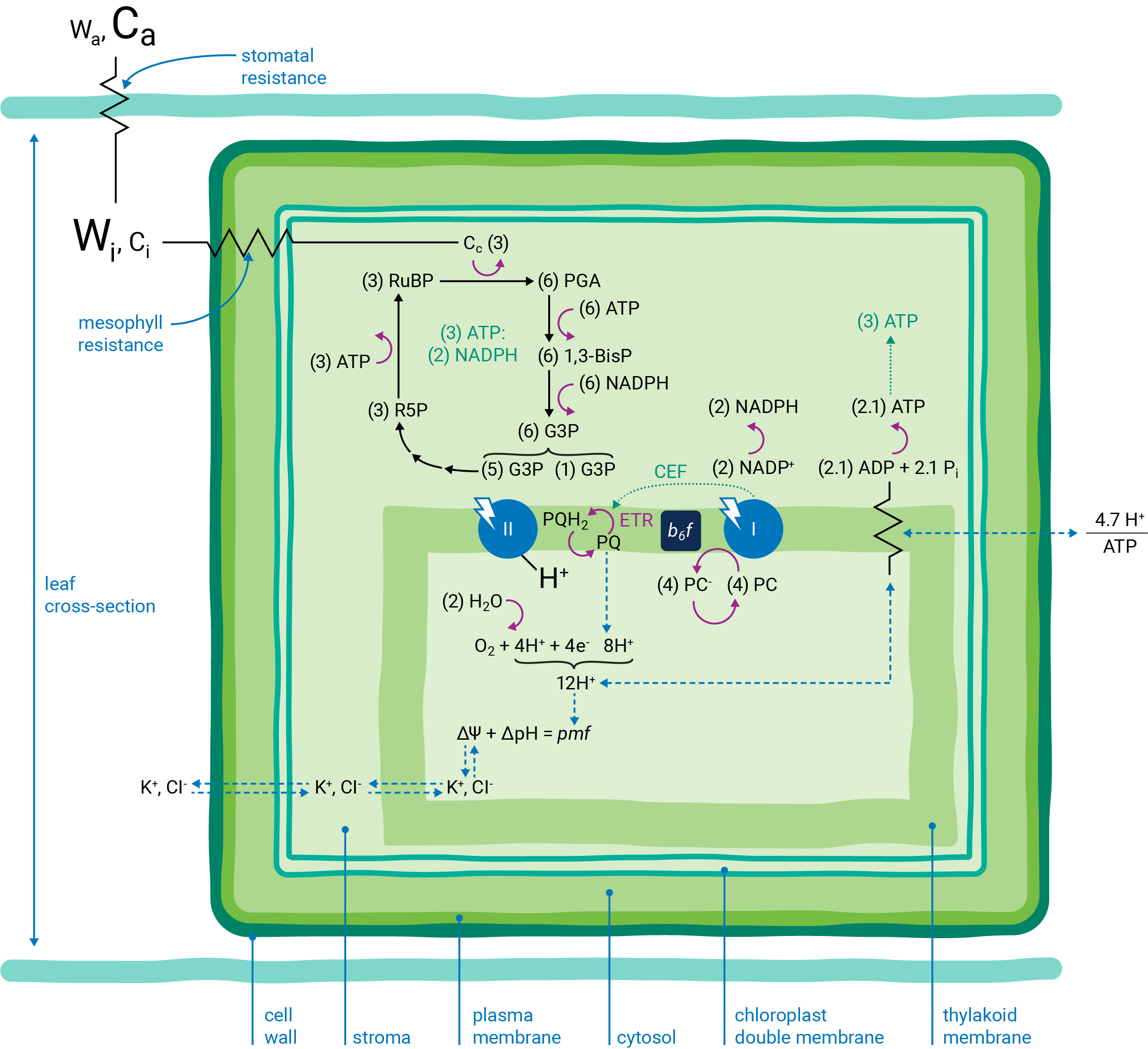
 ) indicate resistance to diffusion. The relative concentrations of gases are indicated by the size of characters.
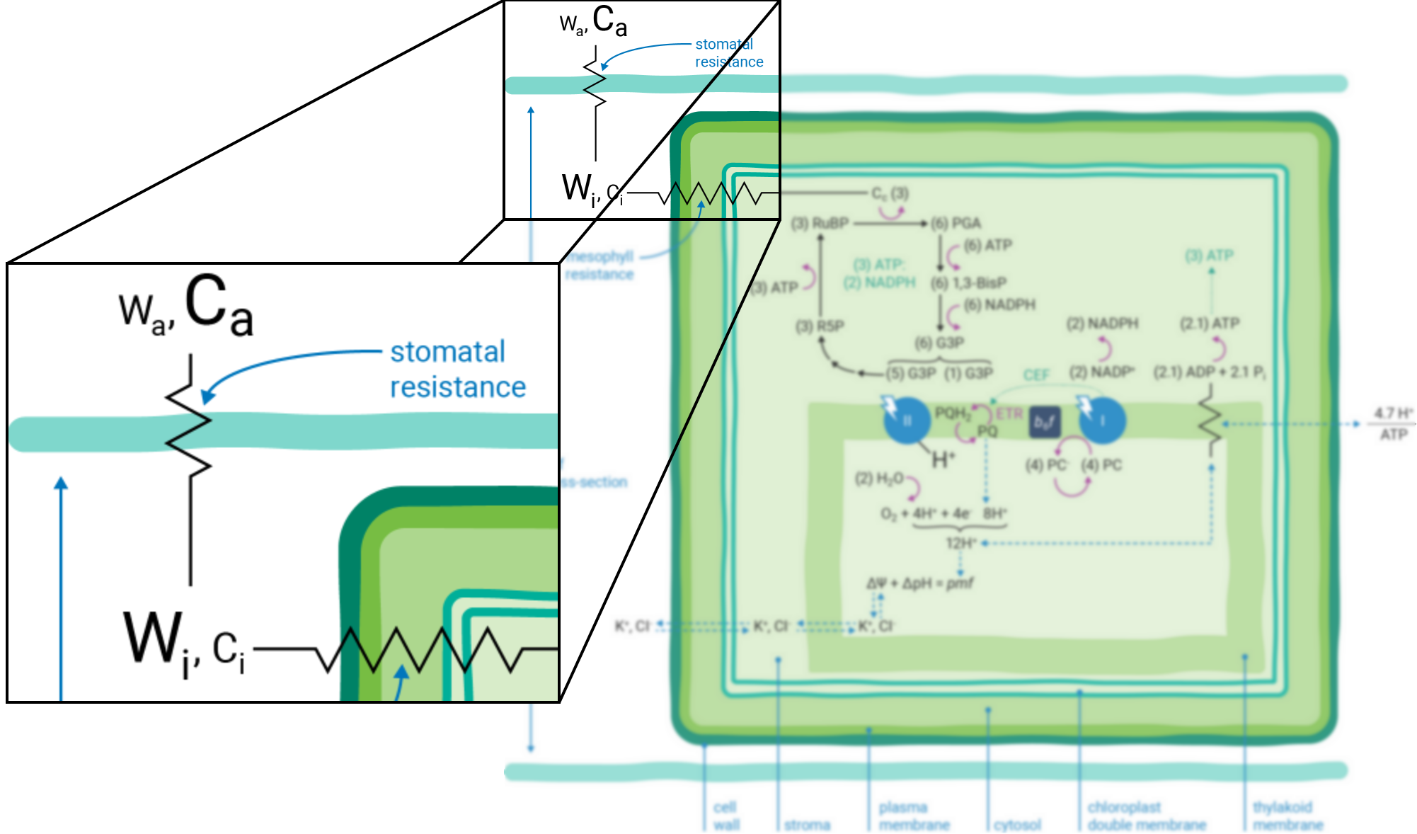
Atmospheric gases (CO2, O2, H2O and others) diffuse into and out of the intercellular leaf air space through stomatal apertures (Figure 9‑2). Stomatal apertures cause resistance to gas diffusion (8). The intercellular air space is assumed to be saturated for water vapor at leaf temperature (9). The relative water vapor concentration within the leaf (Wi) is typically greater than the water vapor concentration in the atmosphere (Wa) as a result of this stomatal resistance. Stomatal resistance also results in a lower CO2 concentration in the leaf intercellular air spaces (Ci) than in the atmosphere (Ca).
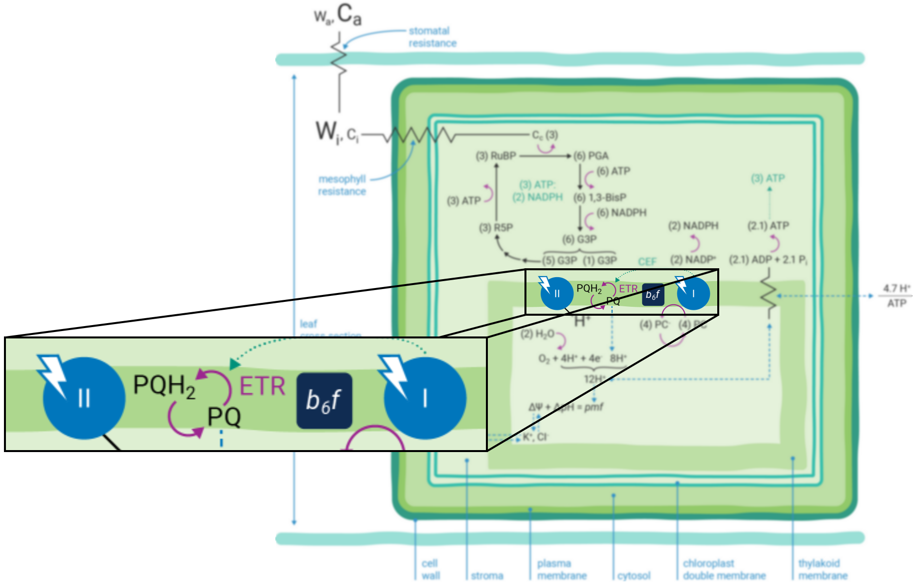
Leaves principally absorb light within the visible region (mostly red and blue) of the electromagnetic spectrum (10). Light absorption, which powers photosynthesis (Figure 9‑3), occurs within specialized pigment-binding protein complexes referred to as photosystems I and II (PSI and PSII) (11). These photosystems are localized within the chloroplast thylakoid membranes (12) and they function in series to facilitate linear electron transfer (ETR; µmol electrons m-2 s-1). Linear ETR is a proton-coupled process (13, 14) that establishes a trans-thylakoid proton motive force (pmf) consisting of both electric field (ΔΨ) (15) and pH (ΔpH) gradients (16).
Photosynthesis-driven transpiration begins with evaporation of H2O from cell wall orifices and into leaf intercellular air spaces (17). Transpiration moves H2O from below-ground soil sources to the atmosphere, transporting ions (e.g., K+ and Cl-, etc.) (18) throughout the plant. These ions serve many cellular purposes including regulation of the relative partitioning of the pmf into ΔΨ and ΔpH components (16, 19).
Energy producing and consuming reactions
The energy producing (i.e., NADPH and ATP formation) and consuming (CO2 assimilation, etc.) reactions of photosynthesis are tightly coordinated (20). The tight coordination is a function of the rigid stoichiometric relationships of key steps within the series of photosynthetic reactions. Assuming 100% quantum conversion at PSI and PSII (21), absorption of four photons at each photosystem results in the net oxidation of two H2O molecules, thereby releasing four protons (H+) into the thylakoid lumen and the generation one molecule of O2 (Figure 9‑1). The electrons freed during these thermodynamically favorable reactions can be subsequently used to form two molecules of NADPH. This transfer of electrons is a somewhat more explicit description of linear ETR.
If the Q-cycle at the cytochrome b6f complex operates constitutively (14, 22 - 24), oxidation of two H2O molecules would result in the net accumulation of twelve protons in the thylakoid lumen, thereby contributing to the pmf (13). The resulting amount of ATP generated as these twelve protons move down their electrochemical gradient through the chloroplast ATP synthase is determined by the enzyme’s H+/ATP ratio (25). The ATP synthase imposes a resistance to proton efflux from the lumen to the stroma of the chloroplast (Figure 9‑4) (6). The H+/ATP ratio of the ATP synthase is contested (26), but if the ratio is four, movement of twelve protons through the ATP synthase would result in the formation of three ATP molecules. Thus, oxidation of two H2O molecules would result in two NADPH and three ATP molecules, precisely the chemical stoichiometry needed to assimilate a single CO2 molecule (7).
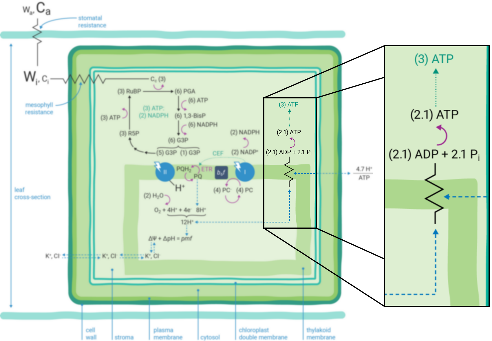
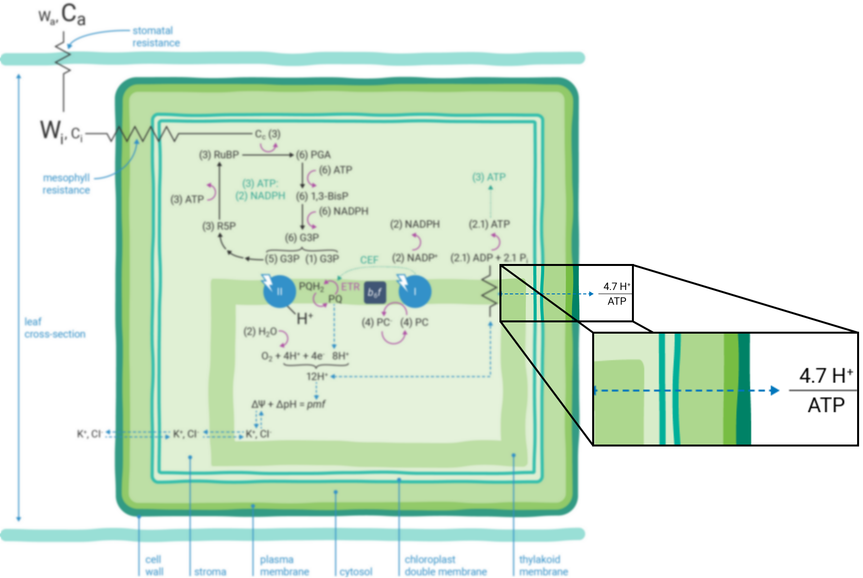
In contrast, given the putative c-subunit composition of the chloroplast ATP synthase (27) (Figure 9‑5), an H+/ATP ratio of 4.7 has been suggested. The net result is a deficit in the amount of ATP produced by linear ETR alone in comparison to that needed to balance the ATP:NADPH ratio for CO2 assimilation alone. Cyclic electron transfer (ETR) around PSI has been suggested as a mechanism for augmenting the pmf, thereby accounting for the deficit of ATP produced by linear ETR (28, 29). The rate of cyclic ETR around PSI needed to accommodate for the short fall in ATP formation has been suggested to be about 12% of linear ETR (26).
In either case, the relationship between linear ETR and the rate of CO2 assimilation is predicted to have a ratio of slightly more than four under conditions when CO2 assimilation is the predominant sink for ATP and NADPH (30). Such conditions occur when photorespiration is inhibited by performing experiments on C4 plants or, under low O2, on C3 plants.
Photosynthetic light reactions must be highly adaptive to a dynamic environment to coordinate the energetic demands for ATP and NADPH while simultaneously regulating light capture (31). Processes other than CO2 assimilation (such as photorespiration, nitrogen and sulfur metabolism) have different ATP and NADPH requirements. Non-photochemical quenching (NPQ) of excess absorbed light energy serves as a photo-protective mechanism (32, 33, 34), preventing formation of highly reactive forms of oxygen: singlet oxygen (1O2) and the superoxide radical anion (O2-).
Energy-dependent quenching (qE) (35), the predominant component of NPQ, is a dual function of the ΔpH component of the pmf (32). The ΔpH both 1) activates a thylakoid lumen-localized enzyme violaxanthin de-epoxidase, which converts violaxanthin (V) to zeaxanthin (Z) in the PSII antenna (36); and 2) regulates protonation of thylakoid lumen-exposed, amino acid residues associated with PSII proteins (37, 38).
Dynamic coordination of the light reactions is required to meet the energetic and photoprotective demands during fluctuating biochemistries that occur during environmental stress, such as drought, for example (6, 31). The coordination is mediated by changes in cyclic ETR around PSI and changes in the proton conductance of the chloroplast ATP synthase (gH+) (19, 39). The former is thought to be predominantly involved in regulating the output ratio of ATP:NADPH, while the latter is thought to be primarily responsible for modulating qE sensitivity (6, 31).
Energy production and photoprotection
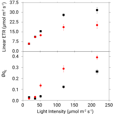
Under fluctuating biochemical demands, qE sensitivity refers to a relative increase in the amount of qE at a given flux of linear ETR (19, 40). Linear ETR and qE increase in hyperbolic and sigmoid manners, respectively, with increasing light intensity under ambient CO2 and 21% O2 (Figure 9‑6, black squares), as well as under 50 ppm CO2 and 21% O2 (Figure 9‑6, red circles). The lower CO2 concentration artificially imposes a change in biochemical demand that mimics various environmental stresses. At the highest light intensity, lowering the CO2 concentration decreased linear ETR by 42% in comparison to values under ambient CO2, whereas qE increased by approximately 2-fold under the same low CO2 concentration treatment. In essence, qE became more sensitive to linear ETR in response to the diminished biochemical demand. Combining analyses of electron and proton transfer reactions of photosynthesis has previously shown that changes in qE sensitivity are predominantly attributable to proportional changes in gH+ (19, 40).
Coordination of assimilation and transpiration
Optimal assimilation of CO2 from the atmosphere by leaf-level photosynthesis is directly coupled with H2O loss. Energy use from light capture, carbon assimilation, and H2O loss is coordinated through regulation of stomatal conductance (gs) (8) and mesophyll conductance (gm) (41 - 45). Research into understanding the inter-dependencies of these regulatory mechanisms has led to interest in selecting for plants to increase the gm:gs ratio, the result of which could lead to more water use efficient plants (46).
Assessing the gas exchange parameters
The gas exchange model described below assumes that the system has no leaks and that air is perfectly mixed in the chamber. In practice, this does not always happen. We present a detailed description of the computations when these assumptions are not met in Mass balance derivation using a two-compartment model.
An open gas exchange system
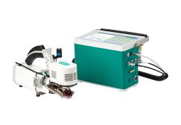
The LI-6800 is an open gas exchange system (9) that measures many parameters needed to estimate photosynthetic gas exchange. The gas exchange system measures the flow rate (µmol air s-1) entering the leaf chamber (µo) and the CO2 and H2O concentrations entering (c0 and w0, respectively) and exiting (ca and wa, respectively) the leaf chamber (Figure 9‑7).
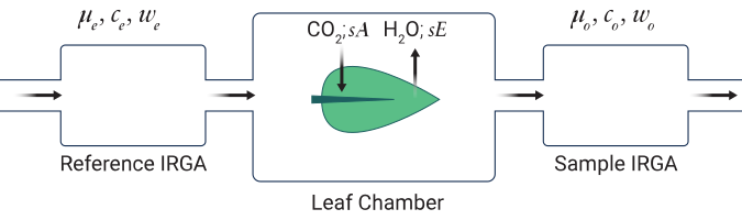
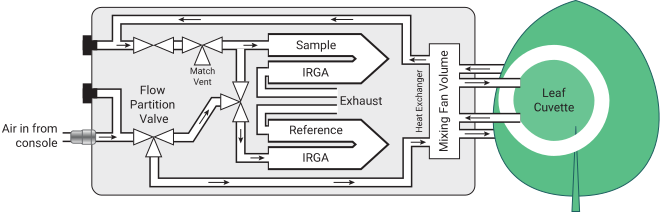
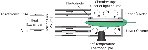
The LI-6800 computes the mass flow per time (i.e., µmol CO2 s-1 and mmol H2O s-1) of these gases into and out of the chamber. The differences between the CO2 and H2O concentrations into and out of the leaf chamber are due to leaf-level CO2 assimilation and transpiration on a leaf area (s) basis (µmol CO2 m-2 s-1 and mmol H2O m-2 s-1). During photosynthetic carbon assimilation (A), the leaf takes up CO2 from the air entering the chamber while simultaneously releasing H2O via transpiration (E) into the chamber air. While the flow rate of air coming out of the chamber (µa) is not directly measured, it is assumed to be:

where s represents leaf area. Transpiration from the leaf is adding water vapor to the chamber, which changes the air density and therefore is added to the total flow into the leaf chamber.
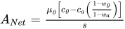
The open-system measurements can subsequently be used to estimate important gas exchange parameters (9, 47). Transpiration, on a leaf area (s) basis, is calculated as:

We can rearrange equations 9‑1 and 9‑2 to give:
9‑3

Similarly, we compute net CO2 assimilation (ANet) (47, 48) as:
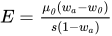
Using equation 9‑1, equation 9‑4 rearranges to:
9‑5

The cascade of derived parameters
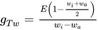
In accordance with reasonable assumptions (9), we use E to derive an expression that represents the total conductance of a leaf to water vapor flux (gTw):
In general, transpiration comes from stomata located on both sides of the leaf. On each side, water vapor diffuses through the stomata and then through the boundary layer to the mixed atmosphere. For each side of the leaf, total resistance to water vapor diffusion (rw) is the sum of stomatal resistance (rsw) plus boundary layer resistance (rbw). So,
9‑7
and
9‑8

for lower (l) and upper (u) leaf surfaces, respectively. We assume boundary layer resistance is the same on both sides of the leaf, so rbw =  =
=  . We define a stomatal ratio:
9‑9

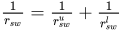
Total stomatal resistance is a parallel combination of stomatal resistances from the upper and lower surfaces, so
9‑10

Total conductance measured by equation 9‑6 represents a parallel combination of series resistances from the upper leaf surface and lower leaf surface, so
9‑11
 ,
,
since gi = 1/ri. From these relationships it can be shown that
9‑12
 .
.
Or, in terms of conductances,
9‑13
 .
.
Solving for gsw yields:
9‑14
 .
.
Similarly, for conductance to CO2,
9‑15

where 1.6 is the ratio of the diffusivities of CO2 to water vapor in air and 1.37 is the same ratio in the boundary layer.
Lastly, we give an expression for Ci (9):

It should be noted that equation 9‑16 is derived from the compilation of many fundamental parameters measured by the LI-6800 gas exchange system.
The Farquahar-von Caemmerer-Berry model
Development of the Farquhar-von Caemmerer-Berry (FvCB) model of photosynthesis (47) was made possible with the types of above-mentioned measured and derived parameters. The general form of the FvCB model is (48, 51):
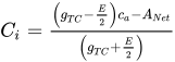
Equation 9‑17 expresses ANet as a function of the minimum rate of photosynthesis that can be supported by: 1) RuBisCO activity (wc); 2) energetic chemical-intermediate (i.e., ATP and NADPH) production for ribulose 1,5-bisphosphate (RuBP) regeneration (wj); and 3) triose phosphate export and utilization (wp). The CO2 compensation point in the absence of day respiration (Γ*) and day respiration (Rd) are routinely estimated from literature sources but can also be measured (52). While expressions for all three potentially limiting processes can be more fully defined (51), we will focus on the RUBP-regeneration limited expression because it directly links measurements of linear ETR and A. The full expression for RUBP-regeneration limited photosynthesis is (48, 51):

J is the electron transport rate needed to supply energy for carboxylation and oxygenation reactions catalyzed by RuBisCO. We’ll say more about J below. The coefficients 4 and 8 can be altered depending upon the assumptions about the relative energy demands for ATP and NADPH (51).
Equation summary
The LI-6800 measures and computes the following parameters related to leaf-level gas exchange measurements.
Light
The photosynthetic photon flux density (PPFD) readings Qin and Qout are computed from
9‑19

9‑20
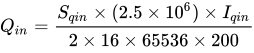
where Sqin and Sqout are the calibration factors, and Iqin and Iqout are the raw counts from the A/D converter.
Leaf temperature
Leaf temperatures Tl1, Tl2 (°C) for the two thermocouples are computed from signals Vl1 and Vl2 (mV) by
9‑21

9‑22

where Tj1 and Tj2 are junction temperatures (°C).
Pressure
Atmospheric pressure Pa (kPa) is reported directly from the on-board sensor.
Chamber over-pressure ΔPc (kPa) is computed from
9‑23

where Vp is the signal from the differential pressure sensor (in V, but taken to be kPa) Vpo is the calibration zero for the sensor, G is fan speed (rpm), F is flow rate, and pca and pcb are empirical coefficients that depend on chamber type (Table 9‑1).
Flow
The flow F (µmol s-1) to the leaf chamber is computed from
9‑24

where af1...af7 are factory calibration constants, Vf is flow meter signal (V), Vfo is calibration zero, and Tk is IRGA block temperature.
Reference and sample IRGA cell flows Fr and Fs (µmol s-1) are computed from
9‑25

9‑26

where Vfr and Vfs are cell exit flow sensor voltage, Vfro and Vfso are the offset value of that voltage, and ar1...ar4 and as1...as4 are factory calibration coefficients.
CO2
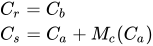
Reference and sample CO2 concentrations Cr and Cs are given by
9‑27

where Mc() is the CO2 match correction function:
9‑28
9‑29

9‑30

where αcr and αcs are absorptances, Pa is atmospheric pressure, Tr and Ts are the cell inlet temperatures, fc is a 5th order polynomial with coefficients (br1...br5 or bs1...bs5) determined at the factory, Scro; Scso and Scr1; Scs1 are the span1 and span2 user calibration settings, Wa and Wb are water concentrations, Xo is the oxygen concentration in percent. Ѱc is the band broadening function for the effect of water and oxygen on CO2, given by
9‑31

where Bwc and Boc are the band broadening coefficients for H2O and O2 respectively on CO2.
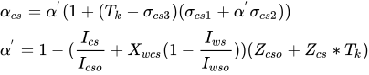
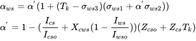
Reference and sample absorptances αcr and αcs are corrected for zero drift with temperature, span drift with temperature, and cross sensitivity with water.
9‑32

9‑33
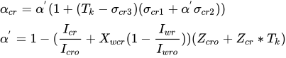
where cr1...cr3 and cs1...cs3 are empirical coefficients for CO2 absorptance span drift determined during calibration, Icr, Icro, Ics, and Icso are the raw IRGA detector absorbing and non-absorbing readings for CO2, and Iwr, Iwro, Iws and Iwso are those for water. Xwcr and Xwcs are empirical cross sensitivity coefficients for water on CO2 determined during calibration, Zcro and Zcso are the current user CO2 zero factors, and Zcr and Zcs are the factors for CO2 zero drift with temperature, determined during calibration.
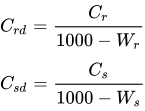
Dry mole fractions Crd and Csd are computed from
9‑34
H2O
Reference and sample H2O concentrations Hr and Hs are given by
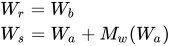
9‑35
where Mw() is the H2O match correction function:
9‑36
9‑37
9‑38

where αwr and αws are the reference and sample absorptances, fw is a 3rd order polynomial with coefficients (dr1...dr3 and ds1...ds3) determined at the factory, Swro, Swr1 and Swso, Sws1 are the H2O span1 and span2 user calibration settings for reference and sample, Ѱo is the band broadening function for the effect of oxygen on H2O, given by
9‑39

where Bow1 and Bow2 are empirical coefficients.
Absorptances αwr and αws are corrected for zero drift with temperature, span drift with temperature, and cross sensitivity with water.
9‑40

9‑41
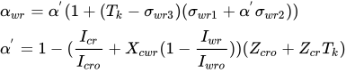
where wr1...wr3 and ws1...ws3 are empirical coefficients for H2O absorptance span drift determined during calibration. Xcwr, Xcws are empirical cross sensitivity coefficients for CO2 on H2O determined during calibration, Zwro and Zwso are the current user H2O zero factors, and Zwr and Zws are the factors for H2O zero drift with temperature, determined during calibration.
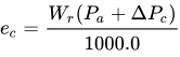
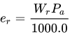
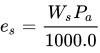
The vapor pressure (kPa) of the air in the reference and sample cells er and es is given by
9‑42
9‑43
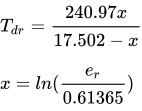
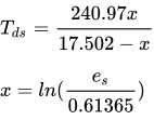
Reference and sample cell dew point temperatures Tdr and Tds are given by
9‑44
9‑45
Humidity indicators
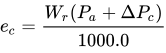
The leaf chamber vapor pressure ec (kPa) is given by
9‑46
The saturation vapor pressure esc in the leaf chamber is a function of chamber air temperature Ta:
9‑47
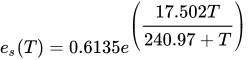
where es(T) is the saturation vapor pressure function:
9‑48

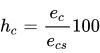
The relative humidity hc (%) in the leaf chamber is given by
9‑49
The vapor pressure deficit of the leaf eΔl is computed from
9‑50
where Tl is leaf temperature ().
Transpiration
The mass balance of water vapor in an open system is given by

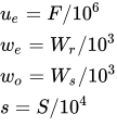
where s is leaf area (m2), E is transpiration rate (mol H2O m-2 s-1), ue and uo are incoming and outgoing flow rates (mol s-1) from the chamber, and we and wo are incoming and outgoing water mole factions (mol H2O (mol air)-1). Since

we can write
9‑53

which rearranges to

The relationships between the terms in equations 9‑51 through 9‑54 and what the LI-6800 measures are
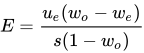
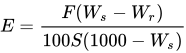
where F is air flow rate (µmol s-1), Ws and Wr are sample and reference water mole fractions (mmol H2O (mol air)-1), and S is leaf area (cm2). The equation that the LI-6850 uses for transpiration is thus
9‑56
Stomatal conductance
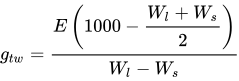
The total conductance gtw of the leaf to water vapor is
9‑57
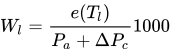
where Wl is the molar concentration of the water vapor within the leaf (mmol H2O (mol air)-1), which is computed from the leaf temperature Tl (°C) and the total atmospheric pressure in the leaf chamber
9‑58
We assume that the total resistance for the upper ru or lower rl surface of a leaf is the sum of the stomatal resistance rs and boundary layer resistance rb of that surface
9‑59
9‑60

and that the upper and lower boundary layer resistances are the same
9‑61
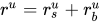
and we define K to be the ratio of stomatal resistances of the two sides

Leaf stomatal resistance rs is given by
9‑63

9‑64
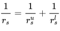
9‑65
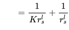
9‑66
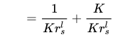
Total conductance g (the inverse of the total resistance r) can thus be written
9‑67
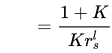
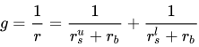
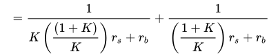
For water vapor, the total conductance gtw is related to stomatal conductance gsw and one sided boundary layer conductance gbw by
9‑70

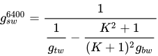
Solving equation 9‑68 for gsw yields
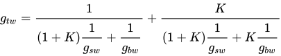
Note that although we defined K to be a particular ratio of upper to lower stomata resistances (equation 9‑62), since K appears as  , we get the same mathematical result if we had defined it the other way. In other words, K is equivalent to 1/K. Note also that the LI-6400 does not use equation 9‑71, but rather a simplified approximation:
9‑72

Boundary layer
The one sided boundary layer conductance to water vapor gbw for a broadleaf is a function of fan speed G (rpm) and leaf area S (cm2).
9‑73
where f is
9‑74

and s is forced to be
9‑75

The empirical coefficients co...c4, reference pressure Po, and leaf area limits Smin and Smax depend on chamber type.
| Chamber | co | c1 | c2 | c3 | c4 | Po | Smin | Smax |
|---|---|---|---|---|---|---|---|---|
| 6800-01 Flr | 0.250 | 0.35860 | -4.01816E-3 | 0.00451074 | -0.0044762 | 96.9 | 1 | 6 |
| 6800-01A 6 cm2 | 0.578 | 0.5229739 | 3.740252E-3 | -6.197961E-2 | -5.608586E-3 | 96.9 | 1 | 6 |
| 6800-01A 2 cm2 | 0.572 | 0.3872742 | -1.870584E-2 | 0.0 | -7.37389E-3 | 96.9 | 1 | 2 |
| 6800-12 3x3 | 0.500 | 0.44869569 | 1.9000035E-3 | -4.26088781E-2 | -3.456516E-3 | 96.7 | 2 | 9 |
| 6800-12A 9 cm2 | 0.579 | 0.3210639 | -1.109987E-3 | 5.106816E-3 | -3.283688E-3 | 96.7 | 2 | 9 |
| 6800-12A 6 cm2FB | 0.345 | 0.552336 | -4.7985e-3 | 0.0 | -7.3557e-3 | 96.7 | 1 | 6 |
| 6800-12A 6 cm2SS | 0.418 | 0.5145466 | -2.5106E-3 | 0.0 | -8.1206E-3 | 96.7 | 1 | 6 |
| 6800-12A 3 cm2FB | 0.188 | 0.5795409 | -1.15295E-2 | 0.0 | -9.7259E-3 | 96.7 | 1 | 3 |
| 6800-12A 3 cm2SS | 0.141 | 0.5263354 | -1.27376E-2 | 0.0 | -1.10157E-2 | 96.7 | 1 | 3 |
| 6800-13 6x6 | 0.430 | 0.267827 | -1.164018E-4 | 2.248202E-3 | -5.109462E-3 | 96.8 | 6 | 36 |
Net assimilation
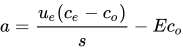
The mass balance of CO2 in an open system is given by
9‑76
where a is assimilation rate (mol CO2 m-1 s-1), ce and co are entering and outgoing mole fractions (mol CO2 (mol air)-1). Using equation 9‑52, we can write
9‑77

which rearranges to

To write equation 9‑78 in terms of what the LI-6800 measures, we use equations 9‑55 and
9‑79
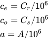
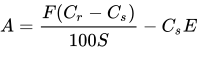
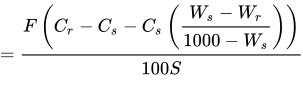
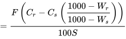
where Cr and Cs are sample and reference CO2 concentrations (µmol mol-1), and A is the net assimilation by the leaf (µmol m-2 s-1). Substitution yields
9‑80
9‑81
9‑82
Intercellular CO2
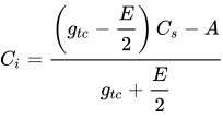
The intercellular CO2 concentration Ci (µmol CO2 (mol air)-1) is given by
9‑83
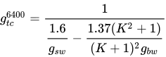
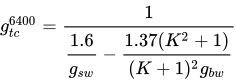
where gtc is the total conductance to CO2. From equation 9‑69, we can write
where 1.6 is the ratio of the diffusivities of CO2 and water in air, and 1.37 is the same ratio for the boundary layer. This is another departure from the LI-6400, which does not use equation 9‑84, but a simplified approximation
9‑85

Energy balance
The LI-6800 provides several potential sources for leaf temperature: it can be directly measured with some combination of the two leaf thermocouples (Tl1 and Tl2), or computed indirectly from a leaf energy balance (Teb). The user can specify what combination to use via three weighting factors fT1, fT2, and fTeb:
9‑86
The energy balance temperature Teb assumes that the energy balance of a leaf in the chamber has three components: net radiation R (W m-2), sensible heat flux H (W m-2), and latent heat flux L (W m-2), and that they all sum to zero:

We consider two components of net radiation: short wave (visible and near IR) and thermal.

where Rabs is absorbed short wave, and Rnt is net thermal. The absorbed short wave radiation is computed by
9‑89

where Qabs is the absorbed irradiance by the leaf (µmol m-2 s-1), and k is the conversion factor for transforming (µmol m-2 s-1) to (W m-2), based on the spectral characteristics of the light source.
The net thermal balance is based on the leaf temperature Tl and the surrounding chamber wall temperature Tw, so the total radiation balance R can be written as

where ϵ is the thermal emissivity of the leaf (usually assumed to be 0.95), and σ is the Stefan-Boltzmann constant (5.67 × 10⁻⁸ W m-2 K-1). The 2 in equation 9‑90 accounts for both sides of the leaf. Wall temperature Tw is not measured, but depends on a user-specified offset ΔTw from chamber air temperature.
9‑91

The latent heat flux L is the transpiration rate E converted to W m-2.
9‑92

The sensible heat flux H is a function of the leaf - chamber air temperature difference Tl−Ta, the specific heat capacity of the air cp (29.3 J mol-1 K-1) and the one sided boundary layer conductance for heat transfer of the leaf gbh, which is 0.92 times the boundary layer conductance for water vapor gbw.
9‑93

9‑94

Equation 9‑87 becomes:

If we let ΔT = Tl − Ta, and note for small ΔT

Substituting equation 9‑96 into 9‑95 and solving for ΔT yields
9‑97

The energy balance leaf temperature Teb is then
9‑98

Sensor head calibration coefficients
| Symbol | Description | XML Locator (/licor/li6850/...) |
|---|---|---|
| af1...af7 ar1...ar4 as1...as4 |
Main flow sensor Ref flow sensor Sample flow sensor |
../factory/flowmeter/a...g ../factory/irga_a/flow/a1...a4 ../factory/irga_b/flow/a1...a4 |
| Bwc Boc Bow1, Bow2 |
Band broadening coefficient for water on CO2 Band broadening coefficient for oxygen on CO2 Band broadening correction for oxygen on water |
../factory/bb/ch ../factory/bb/cx ../factory/bb/hx0, hx1 |
| br1...br5 bs1...bs5 |
Reference CO2 calibration coefficients Sample CO2 calibration coefficients |
../factory/irga_b/co2/a1...a5 ../factory/irga_a/co2/a1...a5 |
| dr1...dr3 ds1...ds3 |
Reference H2O calibration coefficients Sample H2O calibration coefficients |
../factory/irga_b/h2o/a1...a3 ../factory/irga_b/h2o/a1...a3 |
| mco...mc3
mwo...mw3 |
CO2 match coefficients H2O match coefficients |
../cfg/match/co2_adj ... co2 adj 3 ../cfg/match/h2o_adj ... h2o adj 3 |
| pca
pcb |
Pressure correction or fan speed and flow rate Pressure correction or fan speed and flow rate |
../factory/chamber/pca ../factory/chamber/pcb |
| σcr1...σcr3
σcs1...σcs3 σwr1...σwr3 σws1...σws3 |
CO2 reference absorptance span drift with temp CO2 sample absorptance span drift with temp H2O reference absorptance span drift with temp H2O sample absorptance span drift with temp |
../factory/irga_b/co2/s1...s3 ../factory/irga_a/co2/s1...s3 ../factory/irga_b/h2o/s1...s3 ../factory/irga_a/h2o/s1...s3 |
| Scro
Scr1 Scso Scs1 |
Span1 for reference CO2 Span2 for reference CO2 Span1 for sample CO2 Span2 for sample CO2 |
../cal/co2bspan1 ../cal/co2bspan2 ../cal/co2aspan1 ../cal/co2aspan2 |
| Sqin
Sqout |
In-chamber light sensor cal External quantum sensor cal |
../cfg/ppfdin/mult ../cfg/ppfdout/mult |
| Swro
Swr1 Swso Sws1 |
Span1 for reference H2O Span2 for reference H2O Span1 for sample H2O Span2 for sample H2O |
../cal/h2obspan1 ../cal/h2obspan2 ../cal/h2oaspan1 ../cal/h2oaspan2 |
| Vfo
Vfro Vfso |
Zero offset for main flow meter Zero offset for reference flow meter Zero offset for sample flow meter |
../cal/flowmeterzero ../cal/flowbzero ../cal/flowazero |
| Vpo | Zero parameter for differential pressure sensor | ../cal/chamberpressurezero |
| Xo | Oxygen concentration, percent | ../factory/cal/oxygen |
| Xcwr
Xcws Xwcr Xwcs |
Cross sensitivity, CO2 on H2O, reference cell Cross sensitivity, CO2 on H2O, sample cell Cross sensitivity, H2O on CO2, reference cell Cross sensitivity, H2O on CO2, sample cell |
../factory/irga_b/xhc ../factory/irga_b/xch ../factory/irga_a/xhc ../factory/irga_a/xch |
| Zcr
Zcro Zcs Zcso |
Zero drift with temperature for reference CO2 Zero offset for reference CO2 Zero drift with temperature for sample CO2 Zero offset for sample CO2 |
../factory/irga_b/z ../cal/co2bzero ../factory/irga_a/z ../cal/co2azero |
| Zwr
Zwro Zws Zwso |
Zero drift with temperature for reference H2O Zero offset for reference H2O Zero drift with temperature for sample H2O Zero offset for sample H2O |
../factory/irga_b/z ../cal/h2obzero ../factory/irga_a/z ../cal/h2obzero |
Sensor measurements and computations
| Symbol | Description (units) | Name (Label) | Group |
|---|---|---|---|
| αcr
αcs αwr αws |
Reference cell CO2 absorptance Sample cell CO2 absorptance Reference cell H2O absorptance Sample cell H2O absorptance |
abs_c_b abs_c_a abs_h_b abs_h_a |
Raw Raw Raw Raw |
| co...c4 | Boundary layer function coeffs | blc_a...blc_e | ChambConst |
| Ca
Cb Cr Crd Cs Csd ∆Pc |
Sample cell CO2, not adjusted for match Sample cell CO2 (µmol mol−1) Reference cell CO2 (µmol mol−1) Reference cell CO2, dry mole fraction Sample cell CO2 (µmol mol−1) Sample cell CO2, dry mole fraction Chamber over pressure (kPa) |
CO2_a CO2_b CO2_r CO2_r_d CO2_s CO2_s_d Pchamber (∆Pcham) |
Meas Meas2 Meas Meas Meas Meas Meas |
| er
es Icr Icro Ics Icso |
Reference cell vapor pressure (kPa) Sample cell vapor pressure (kPa) Reference CO2 raw detector count Reference CO2 raw detector reference count Sample CO2, raw detector count Sample CO2 raw detector reference count |
e_r e_s Wc_r Wco_r Wc_s Wco_s |
Meas2 Meas2 Raw Raw Raw Raw |
| Iqin
Iqout |
In-chamber PPFD sensor raw counts External quantum sensor raw counts |
||
| Iwr
Iwro Iws Iwso |
Reference H2O raw detector count Reference H2O raw detector reference count Sample H2O raw detector count Sample H2O raw detector reference count |
Ww_r Wwo_r Ww_s Wwo_s |
Raw Raw Raw Raw |
| Pa | Atmospheric pressure (kPa) | Press (Pa) | Meas |
| F
Fr Fs |
Flow to chamber (µmol s−1) Flow from reference cell (µmol s−1) Flow from sample cell (µmol s−1) |
Flow Flow_r Flow_s |
Meas Status Status |
| G | Chamber fan rotation rate (rpm) | Fan speed | Status |
| Qin
Qout |
In-chamber PPFD External PPFD |
PPFD_in (Q_amb_in) PPFD_out (Q_amb_out) |
Meas Meas |
| Ta | Leaf chamber air temperature (C) | Tchamber (Tair) | Meas |
| Tdr
Tds |
Dewpoint temperature reference cell (C) Dewpoint temperature sample cell (C) |
Td_r Td_s |
Meas2 Meas2 |
| Tj1
Tj2 Tk |
Leaf T/C 1 junction temperature (C) Leaf T/C 2 junction temperature (C) IRGA block temperature (C) |
Tleafjunction (Tleaf_j) Tleafjunction2 (Tleaf2_j) Tirga_block (Tirga) |
Status2 Status2 Status |
| Tl1
Tl2 Tr Ts |
Leaf temperature 1 (C) Leaf temperature 2 (C) Reference cell inlet temperature (C) Sample cell inlet temperature (C) |
Tleaf Tleaf2 Tb (Tr) Ta (Ts) |
Meas Meas Status Status |
| Vf
Vfr Vfs |
Signal (V) from main flow sensor Signal (V) from reference flow sensor Signal (V) from sample flow sensor |
Flow Flow_b_v (Flow_r_v) Flow_a_v (Flow_s_v) |
Raw Raw Raw |
| Vl1
Vl2 |
Leaf temperature 1 signal (mV) Leaf temperature 2 signal (mV) |
leaf_t_mv (Tleaf_mv) leaf2_t_mv (Tleaf2_mv) |
Raw Raw |
| Vp | Differential pressure signal (V or kPa) | VPchamber | Raw |
| Wa
Wb Wr Ws |
Sample cell H2O not corrected for match Reference cell H2O Reference cell H2O (mmol mol−1) Sample cell H2O (mmol mol−1) |
H2O_a H2O_a H2O_r H2O_s |
Meas Meas2 Meas Meas |